Network Latency Calculator
Break one-way network latency into its four real components: propagation delay from distance and medium, transmission delay from packet size and link rate, and processing plus queuing delay across each router hop. Enter your path and read the total delay in milliseconds with a full percentage breakdown.
📡Real Network Path Presets
🔢Path and Link Inputs
Physical cable length along the route, not straight-line.
Applies to the distance field above.
Sets the signal propagation speed used for delay.
Frame size on the wire; 1500 is a typical MTU.
Serialization speed of the bottleneck link.
Unit for the link rate value above.
Store-and-forward devices along the path.
Route lookup and forwarding time at each hop.
Wait in buffers; rises sharply under congestion.
Controls rounding on every result card.
⚡Formula Snapshot
📡Propagation Speed by Medium
| Medium | Speed (m/s) | Fraction of c | Delay per km |
|---|---|---|---|
| Vacuum / space | 3.0 × 10^8 | 1.00 c | 3.34 µs |
| Wireless / air | 3.0 × 10^8 | ~1.00 c | 3.34 µs |
| Single-mode fiber | 2.0 × 10^8 | 0.67 c | 5.0 µs |
| Coax / copper | 2.0 × 10^8 | 0.66 c | 5.0 µs |
| Cat-cable copper | 1.9 × 10^8 | 0.64 c | 5.3 µs |
| Satellite RF path | 3.0 × 10^8 | 1.00 c | 3.34 µs |
🌎City to City Fiber Latency Floor
| Route | Fiber Distance | Min One-Way | Notes |
|---|---|---|---|
| New York to Chicago | 1200 km | 6.0 ms | Backbone hop |
| New York to London | 5600 km | 28 ms | Transatlantic |
| London to Frankfurt | 640 km | 3.2 ms | EU core |
| LA to Tokyo | 8800 km | 44 ms | Transpacific |
| Sydney to Singapore | 6300 km | 32 ms | Sea route |
| Mumbai to Marseille | 7100 km | 36 ms | SEA-ME-WE |
| Same metro area | 50 km | 0.25 ms | Metro ring |
| Within one building | 0.1 km | 0.0005 ms | LAN link |
🎮Latency Budget by Application
| Application | Good One-Way | Usable Limit | What Breaks Past It |
|---|---|---|---|
| Competitive gaming | Under 15 ms | 30 ms | Hit registration lag |
| VoIP / video call | Under 75 ms | 150 ms | Talk-over, echo |
| Web browsing | Under 50 ms | 100 ms | Sluggish page loads |
| Live video stream | Under 100 ms | 250 ms | Buffering, drift |
| Financial trading | Under 1 ms | 5 ms | Missed arbitrage |
| Cloud file sync | Under 100 ms | 300 ms | Slow throughput |
📊Medium Comparison Grid
| Medium | Speed Fraction c | Delay per km | Delay 1000 km | Typical Use | Notes |
|---|---|---|---|---|---|
| Single-mode fiber | 0.67 c | 5.0 µs | 5.0 ms | Backbone, metro | Low loss long haul |
| Multimode fiber | 0.67 c | 5.0 µs | 5.0 ms | Data center | Short reach only |
| Coax copper | 0.66 c | 5.0 µs | 5.0 ms | Cable last mile | Shared segment |
| Twisted pair | 0.64 c | 5.3 µs | 5.3 ms | LAN, DSL | Under 100 m runs |
| Terrestrial wireless | 1.00 c | 3.34 µs | 3.34 ms | Microwave, 5G | Line of sight |
| LEO satellite | 1.00 c | 3.34 µs | 3.34 ms | ~550 km orbit | Short RF path |
| GEO satellite | 1.00 c | 3.34 µs | 3.34 ms | ~35786 km orbit | ~120 ms one-way |
⚙Formula Breakdown
💡Latency Tuning Tips
What about email? Send it and watch it vanish. Reply comes back nearly immediatey. Magic! Video chat? Your face locks up when you talk to people on the other side of planet. What’s the difference between them? Speed? Bandwidth? No, that’s latency: the time it takes for one packet of data to get from point A to point B.
The place where that time gets spent is what turns vague frustration into hard-won engineering insight. To make it clear where your performance are being hurt, the calculator splits out one-way delay into its four physical part. Queuing + Processing Delay + Transmission Delay + Propagation Delay.
Understanding What Causes Internet Lag
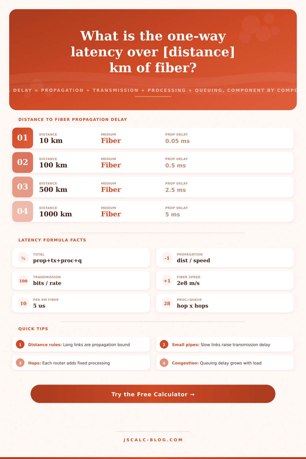
Propagation delay just means how long it takes for signal to spend in flight from source to destination. There’s no getting around this math: Distance/Speed. Optical fiber signals move about two hundred million meters per second. That’s because they’re slowed in glass; they go about two-thirds the speed of light in a vacuum. Fiber adds an average of about five microseconds per kilometer. So two hundred kilometers of cable will take a millisecond one way. You can’t beat that physics.
The delay caused by pushing every bit of a packet onto the wire is known as transmission delay. Also sometimes referred to as serialization delay. It’s fully dependent on link rate and packet size. For example, there are 12,000 bits in an ordinary 1500-byte Ethernet frame. That teeny-weeny fraction would only take 0.012 milliseconds to send across a moddern 1 Gbps connection. But at a poky 1 Mbps uplink, that very same frame would take 12 milliseconds. Since the link is too slow to send the data out, it gets stuffed with raw data, which clogs the works and increases the delay by a thousand times. That’s what makes rural DSL connections feel so sluggish, even over relatively short distances. The traffic jam is the interface itself.
Next are the hidden costs of having all of your packets pass through intermediary machines. Each router inspects header information and selects an outbound port. Each hop typically take a fraction of a millisecond: that’s processing delay. The wild card is queuing delay. If there’s no traffic on a link, packets moves quickly through buffers. But as traffic loads up those queues, they wait longer and longer. Often, the queuing delay itself can surpass the propagation and transmission delays combined.
We model them independently. This makes the responsiveness easy to see, as you can see how much network load contributes directly to your overall delay budget. If you read that as percentages, it tells you precisely where you could do something about it. For example, on a fiber link across a continent, more than ninety per cent is propagation: faster routers won’t help much if at all. You’d need to make the physical route shorter or put some kind of edge cache nearer the user to move the needle. But on a slow last-mile link, maybe it’s all transmission. Now you know where to stop pointing fingers… Because you now know what is congestion-bound and what is physics-bound.
These are very abstract numbers, but these reference tables helps connect them to some sense of real world experience. There’s a 6 millisecond hop from New York to Chicago and 44 milliseconds across to Tokyo. Then there are application budget ranges that differ widely. Web browsing can tolerate up to 100 milliseconds while competitive gaming struggles beyond 30 milliseconds. Even geostationary satellite links will tack on about 120 milliseconds one way just for being thirty-five thousand kilometers out in space. That distance is unavoidable. It travels at the speed of light, but that’s just how far it has to go.
The tool has ten presets for various scenarios… From a low-Earth-orbit Starlink hop to a transatlantic cable to a local LAN run. A quick flick across them illustrates how the dominant component vary with changes in hop count, link rate, and distance. While any one static result can be illuminating, how it reveals the tradeoffs involved in network design makes it more so.
Ping reports twice the one-way delay plus server response time, rather than just the one-way latency. One could argue that this comparison is measuring round-trip instead of just one-way delay. That’s true, but it’s by design. Why? Because Ping reports twice the one-way delay and adds the server response time. It confuses endpoint processing with path physics.
Ping reports half the one-way delay and adds the server response time. It confuses Endpoint processing with Path Physics. Separating these allows you to think clearly about the path first without adding any additional Protocol Overhead. Size your Trading Link, troubleshoot why your Video Call isn’t responding… knowing exactly where the Milliseconds are hiding turns mystery into something we can manage.
There is always delay in the wire. It should of been waiting for you.