Loaded Voltage Divider Calculator

See what a real load does to a resistive divider. Enter Vin, the top resistor R1, the bottom resistor R2, and the load resistance RL, and this tool returns the ideal unloaded Vout, the actual loaded Vout, the voltage droop percent, and the effective bottom resistance R2eff = R2 in parallel with RL, plus a stiffness verdict.

⚡Real Loaded Divider Presets

🔌Divider and Load Inputs

Input voltage Vin (V)

Supply voltage across the whole divider.

Resistor unit

Applies to R1, R2, and RL below.

Top resistor R1

Between Vin and the output tap node.

Bottom resistor R2

Between the tap node and ground.

Load resistance RL

Input impedance of whatever reads the tap.

Define the load by

Current mode derives RL from the loaded tap voltage.

Load current draw (mA)

Used only when the load is defined by current.

Result decimals

Controls rounding on the result cards.

Ideal Unloaded Vout 0 V no load, RL infinite

Actual Loaded Vout 0 V with RL across R2

Voltage Droop 0% drop caused by the load

Effective R2eff 0 R2 in parallel with RL

🔢Formula Snapshot

VunVin R2/(R1+R2)

R2effR2 RL/(R2+RL)

VldVin R2e/(R1+R2e)

StiffR2 <= RL/10

📊Load Ratio vs Droop Percent

RL / R2 Ratio	Droop at Midpoint	Verdict	Meaning
100 : 1	0.99%	Stiff	Load barely felt
50 : 1	1.96%	Stiff	Safe for ADC refs
20 : 1	4.76%	Stiff	Good margin
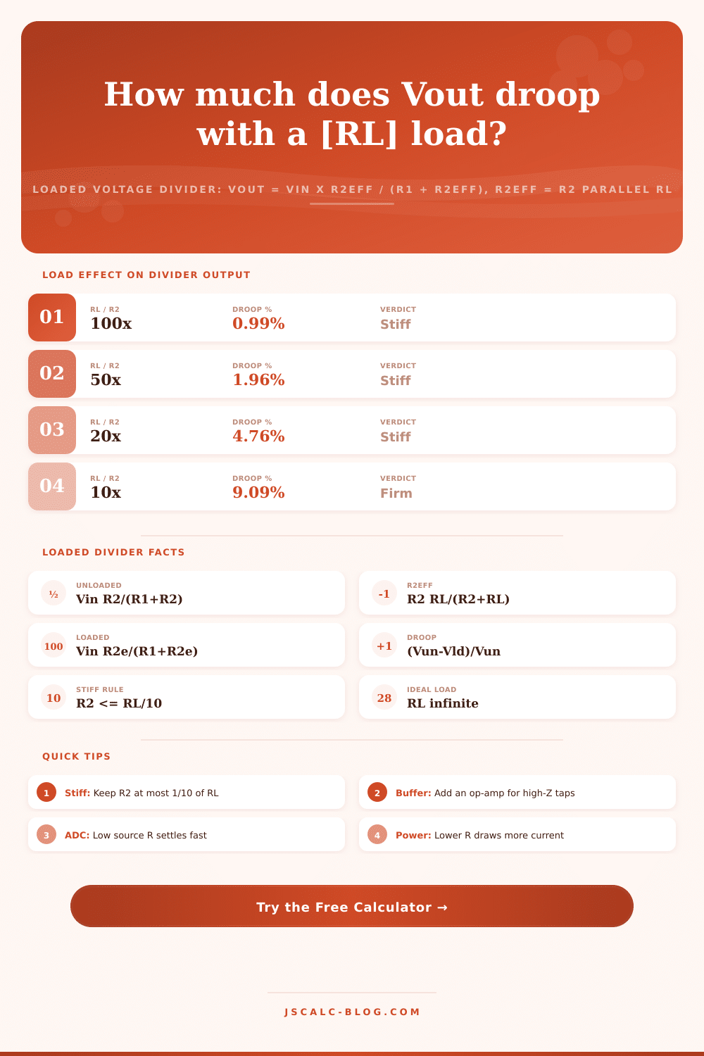
10 : 1	9.09%	Firm	Rule of thumb edge
5 : 1	16.7%	Soft	Noticeable sag
2 : 1	33.3%	Weak	Heavy loading
1 : 1	50.0%	Weak	Half voltage lost
0.5 : 1	66.7%	Weak	Divider overwhelmed
0.2 : 1	83.3%	Weak	Nearly shorted

📏The Stiff Divider Rule (R2 <= RL/10)

Load RL	Max R2 for Stiff	Example R1 : R2	Bleeder Current
1 kΩ	100 Ω	100 Ω : 100 Ω	High, milliamps
10 kΩ	1 kΩ	1 kΩ : 1 kΩ	Moderate
100 kΩ	10 kΩ	10 kΩ : 10 kΩ	Low, microamps
1 MΩ	100 kΩ	100 kΩ : 100 kΩ	Very low
10 MΩ	1 MΩ	1 MΩ : 1 MΩ	Tiny, noise risk
47 kΩ	4.7 kΩ	4.7 kΩ : 4.7 kΩ	Low

🗃Loaded Output Comparison Grid

Vin	R1	R2	RL	Unloaded Vout	Loaded Vout	Droop
12 V	10 kΩ	10 kΩ	100 kΩ	6.000 V	5.714 V	4.76%
5 V	1 kΩ	1 kΩ	100 kΩ	2.500 V	2.488 V	0.50%
3.3 V	10 kΩ	20 kΩ	47 kΩ	2.200 V	1.927 V	12.42%
12 V	4.7 kΩ	4.7 kΩ	10 kΩ	6.000 V	4.858 V	19.03%
9 V	100 kΩ	100 kΩ	10 kΩ	4.500 V	0.750 V	83.33%
5 V	2.2 kΩ	3.3 kΩ	50 kΩ	3.000 V	2.923 V	2.57%
24 V	47 kΩ	10 kΩ	1 kΩ	4.211 V	0.455 V	89.18%
12 V	1 kΩ	2 kΩ	20 kΩ	8.000 V	7.742 V	3.23%
5 V	10 kΩ	10 kΩ	1 MΩ	2.500 V	2.488 V	0.50%
3.3 V	2 kΩ	1 kΩ	50 kΩ	1.100 V	1.089 V	1.00%

⚙Formula Breakdown

Unloaded Vout = Vin R2/(R1+R2)The ideal divider ratio with no load attached. With 12 V, R1 = 10 k, R2 = 10 k this is 12 x 10 / (10 + 10) = 6.000 V.

R2eff = R2 RL/(R2+RL)Attaching the load RL puts it in parallel with R2. With R2 = 10 k and RL = 100 k, R2eff = 10 x 100 / (10 + 100) = 9.091 k.

Loaded Vout = Vin R2eff/(R1+R2eff)Recompute the divider using R2eff instead of R2. Here 12 x 9.091 / (10 + 9.091) = 5.714 V, lower than the ideal 6 V.

Droop % = (Vun − Vld)/Vun x 100The fraction of output lost to loading. (6.000 − 5.714) / 6.000 x 100 = 4.76% droop for this example.

Stiff test: R2 <= RL/10A divider is stiff when the bottom resistor is at most one tenth of the load. 10 k <= 100 k / 10 = 10 k, so this case is right at the stiff limit.

💡Design Tips for Loaded Dividers

Keep the divider stiff: Make the bottom resistor R2 no more than one tenth of the load resistance RL. At a 10 to 1 ratio the droop is about 9 percent, at 20 to 1 it falls to under 5 percent, and at 100 to 1 it is roughly 1 percent. Lower resistor values fight loading better but draw more standing current, so balance accuracy against the milliamps you can spare.

Buffer high-impedance taps: When you truly need large megohm resistors to save power, do not feed a low-impedance load directly. Follow the tap with an op-amp voltage follower, which presents a load of many megohms and drives the next stage from a near-zero output impedance. That gives you the exact unloaded ratio, for example a clean 3.3 V reference, with essentially zero droop regardless of what draws current downstream.

On paper, a voltage divider appears straightforward: Two resistors in series and the output equals Vin times R2 over the total resistance (R1 + R2). True enough, that equation from your textbook, except now put a load across the tap and everything changes. Instantly, the output fall short of the expected value. I’ve seen many newbies puzzled why their “6 V” reference reads “only” 4.9 V on their meter.

Instead of finding out after the board is assembled, let this calculator do math for you, allowing you to see the loading effect. It figures the ideal (unloaded) output, the voltage with the actual load attached, and how much the output have dropped (in percent).

2>Why Your Voltage Divider Loses Power When You Add a Load

Anything drawing current off of the output is a load. It can be another piece of equipment with an input, a transistor base, a pin on an analog-to-digital converter, etc. Think of it as an electrical resistor between the tap and ground, called RL. And RL are directly across the bottom resistor R2.

Two resistors in parallel always combine to something smaller than either one alone. This makes effective bottom resistor smaller. Because the divider ratio depend on the bottom resistor, this makes the output voltage smaller. The larger the load (i.e., the lower its resistance), the more the output will collapse. That’s what most folks miss when they design assuming no-load/open-circuit condition only.

>To achieve this, the tool provides a set of four interrelated equations. It starts with the optimal unloaded case. It then determines the effective bottom resistance by combining RL in parallel with R2. It then recalculates the divider based on the new effective resistance, and finally it shows the droop, or how much the voltage drop between the unloaded and loaded cases as a percentage. This sort of step-by-step dissection isn’t only useful because it makes the math transparent; it also helps explain how it’s all working so you don’t have to take “the answer” at face value. You know why there was a drop, not just what it is.

So let’s say we have R1 and R2 each rated at 10 kilohms, fed from a 12 V supply and carrying a 100 kilohm load. With no load (unloaded), the tap will read a nice clean 6 V. Add your 100 k load and you now has an effective bottom resistance of approximately 9.1 kilohms. Output voltage goes down to 5.714 V, or a drop of about 4.8 percent. Not bad; not something that would of be unacceptable for most applications.

>Replace it with a larger load, such as a heavy 10 k. The effective bottom resistance decreases again, moving the output voltage closer to 4 V. This causes the amount of “droop” to increase to about 33 percent. The divider stays the same, but the outcome is completely different just by changing the load size.

A simple rule of thumb called the stiff divider rule helps engineers manage loading: make the bottom resistor R2 no greater than one tenth of the load resistance RL. If R2 remains below (or equal to) this value, then the parallel combination barely changes, and the droop will remain modest. Increase the ratio to twenty to one, and the droop will be less then five percent. Go to one hundred to one, and it’s nearly one percent. This is the test applied automatically by the calculator, which compares R2 to RL over ten and flags the design either as weak or stiff. It provides an instant judgment of how much margin the design hold.

Occasionally you know that the load demands a certain amount of current from the tap, but not its resistance. The tool takes that as well: just type in the milliamp value instead of the ohm value, and it computes an equivalent RL based on the operating voltage and proceeds with the analysis. That’s useful for situations where a datasheet specifies a particular input bias current (rather than an impedance). Ohmic units include options of ohms, kilohms and megohms; there’s no need to convert manually into whatever scale you’re using on your schematic.

>The presets load real world scenarios that show you some of the potential pitfalls. For example, these include an op-amp bias point with a light load, a sensor divider fighting a heavy load, or an ADC input reading a divider into a 100 k load. These are not only starting points but teaching cases in themselves, showing what a weak divider is and why it’s different than a stiff divider. And you get to see what happens if you change just one resistor.

Resistor options can only solve the problem up to a certain point. No ratio will suffice if you have a low impedance load that needs to be driven but also requires a big resistor for power savings. Then the solution is generally to add an op-amp voltage follower as output of the tap. That presents high impedance at the divider input, and the op-amp provides near zero output impedance into whatever follows. This calculator helps determine the breakpoint. If you have a load with too low an impedance that causes a lot of droop, adding a buffer can help. Do this if lowering the resistor value would waste more current than you want.

Set up the pre-set and tinker with the numbers. Look at how much droop results. Then, off you go designing dividers that don’t lose voltage when you really need them to stay steady.

Loaded Voltage Divider Calculator – Vout Droop Under Load