Gustafson's Law Scaled Speedup Calculator
Estimate the scaled parallel speedup of a program with Gustafson's Law, S(N) = N - (1 - P)(N - 1) = (1 - P) + P times N, where P is the parallel fraction of the scaled workload and N is the processor count. Because the problem grows with the machine, speedup rises almost linearly with no fixed ceiling. Compare it side by side with fixed-size Amdahl to watch the two diverge.
🚀Choose a Mode
🎯Real Scaled Workload Presets
📝Scaling Inputs
Share of the scaled workload that runs in parallel. Serial part is s = 100 - P percent.
Cores, threads, or nodes running the scaled problem in parallel.
Solve mode finds the processor count N needed to reach this speedup at fixed P.
Measured wall time on N processors. Used to estimate the equivalent serial time.
Amdahl assumes a fixed problem, so its speedup caps at 1 / (1 - P).
Controls rounding on every result card.
🔢Formula Snapshot
📊Gustafson Speedup by Parallel Fraction and N
| Parallel P | N = 2 | N = 4 | N = 8 | N = 16 | N = 64 | N = 256 |
|---|---|---|---|---|---|---|
| 50% | 1.50x | 2.50x | 4.50x | 8.50x | 32.50x | 128.50x |
| 75% | 1.75x | 3.25x | 6.25x | 12.25x | 48.25x | 192.25x |
| 90% | 1.90x | 3.70x | 7.30x | 14.50x | 57.70x | 230.50x |
| 95% | 1.95x | 3.85x | 7.65x | 15.25x | 60.85x | 243.25x |
| 99% | 1.99x | 3.97x | 7.93x | 15.85x | 63.37x | 253.45x |
| 99.9% | 2.00x | 4.00x | 7.99x | 15.99x | 63.94x | 255.75x |
🗃Gustafson vs Amdahl Divergence Grid
| Parallel P | N Procs | Gustafson S | Amdahl S | Amdahl Cap | Extra Gain |
|---|---|---|---|---|---|
| 90% | 16 | 14.50x | 6.40x | 10.00x | 8.10x |
| 90% | 256 | 230.50x | 9.66x | 10.00x | 220.84x |
| 95% | 16 | 15.25x | 9.14x | 20.00x | 6.11x |
| 95% | 256 | 243.25x | 18.62x | 20.00x | 224.63x |
| 99% | 64 | 63.37x | 39.26x | 100.00x | 24.11x |
| 99% | 256 | 253.45x | 72.11x | 100.00x | 181.34x |
| 99.9% | 256 | 255.75x | 203.98x | 1000.00x | 51.77x |
| 99.9% | 1024 | 1022.98x | 506.19x | 1000.00x | 516.79x |
⚖Parallel Efficiency Table
| Parallel P | N = 4 | N = 16 | N = 64 | N = 256 |
|---|---|---|---|---|
| 50% | 62.50% | 53.13% | 50.78% | 50.20% |
| 75% | 81.25% | 76.56% | 75.39% | 75.10% |
| 90% | 92.50% | 90.63% | 90.16% | 90.04% |
| 95% | 96.25% | 95.31% | 95.08% | 95.02% |
| 99% | 99.25% | 99.06% | 99.02% | 99.00% |
| 99.9% | 99.93% | 99.91% | 99.90% | 99.90% |
📏Serial Fraction and Percent Reference
| Parallel P | Serial s = 1 - P | As Fraction | Amdahl Ceiling 1/(1-P) |
|---|---|---|---|
| 50% | 50% | 0.50 | 2x |
| 75% | 25% | 0.25 | 4x |
| 90% | 10% | 0.10 | 10x |
| 95% | 5% | 0.05 | 20x |
| 99% | 1% | 0.01 | 100x |
| 99.9% | 0.1% | 0.001 | 1000x |
⚙Formula Breakdown
💡HPC Scaling Tips
Think about how faster machines, double the cores, for example; will speed up your simulations. The classic solution is Amdahl’s Law, which says there is a brick wall defined by fraction of your program that can’t be run in parallel. This is valid reasoning if your program is fixed size. But in today’s world of large-scale computation, the size of the problem expands as the compute power does.
Gustafson’s Law flips this notion on its head: what happens if you increase the size of the problem as well? Then there is no ceiling on speedup which scales almost directly with machine. This website computes that for you. Play around and see how much more efficient you’ll be if you let the problem size grow to match compute resources at hand.
Why Gustafson’s Law Is Better for Big Computers
That’s a fairly simple equation, but one with wide consequences for systems design. You can think about it this way: scaled speedup equals (number of processors), (penalty for serial fraction of code x rest-of-cores). You can also say it this way: (serial part) + ((processor-count) x (parallel-fraction)). Both equations gets you to the same place, just with a slightly different understanding of what might be going wrong.
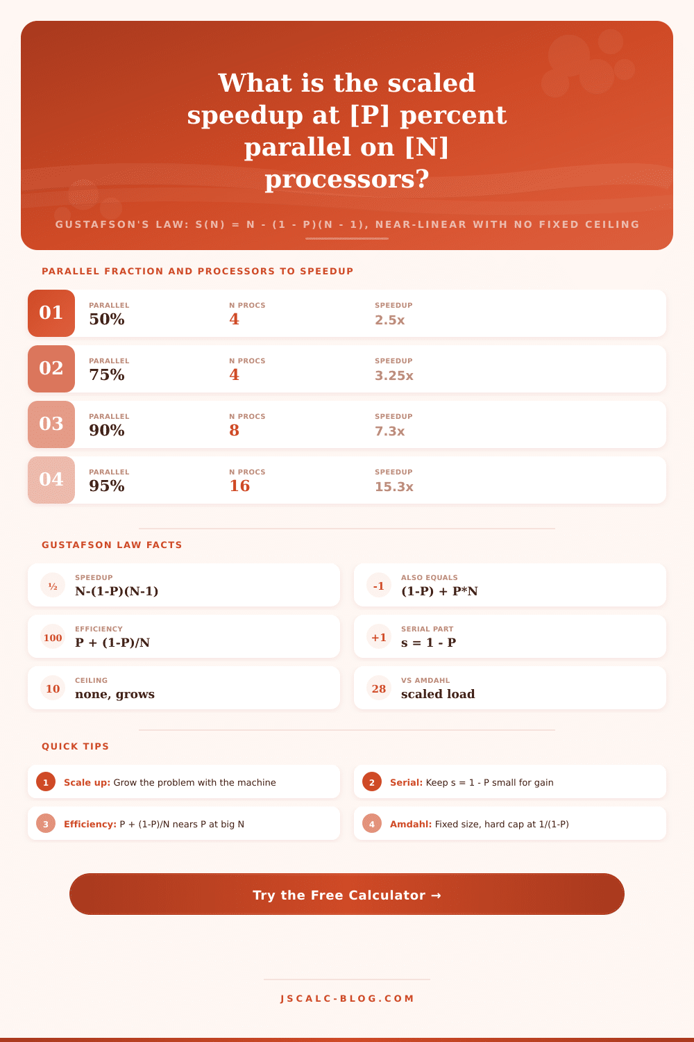
On 16 processors, you have 95% of your scaled workload running in parallel; so the serial slice accounts for five percent. From the speedup calculator, we find speedup of approximately fifteen point two five times, not the expected twenty times. The difference there is the price of code that cannot run in parallel no matter how many core you throw at it.
In that case, our efficiency behaves in an interesting way compared to the traditional scaling laws. Since the parallel work grows along with the machine, the efficiency metric converges towards the parallel fraction from above for increasing processors. As long as the serial part is sufficiently small, hardware use will remain high even on very large clusters. The tool calculates this efficiency and provides it to you automatically.
This allows you to get a clear signal whether you struggle with overhead or not, did your parallelization effort pay off? Does the number go down substantially below the parallel fraction? Then probably the distribution of work over nodes are wrong.
This is unlike Amdahl’s Law, which says supercomputers will hit a hard limit on speedup; instead, Gustafson’s Law explains why they don’t hit diminishing returns and can simply keep getting bigger and faster. In Amdahl’s world, there is a hard upper bound on speedup, determined purely by the amount of serial work in the task. Gustafson’s world assumes an ever-increasing problem size. That removes the limit entirely.
The calculator has a switch for displaying these results side-by-side. The discrepancy becomes obvious. When you have very little parallel work, the difference isn’t big. At high parallel fractions, the difference is staggering: you might get only ten times speedup with Amdahl but over two hundred times with Gustafson on the same hardware configuration.
It’s why we don’t see weather models and fluid dynamics simulations stall when ported to bigger computers. When using the presets, you get an instant idea about what to expect for typical types of work. Database queries may only hit 80 percent parallelism, whereas weather simulations often hit nearly ninety-eight. Why does this matter? These are realistic representations of your code’s architecture instead of theoretical perfection. Over-estimating the parallel fraction leads to overly optimistic estimates of speedup. Under-estimating it risks turning down hardware that could benefit you.
The tool can also be used to solve for processor count. Need a certain amount of speedup by X date? The tool reverses the equation and tells you how many cores you should of provision.
But more than math, this shows the power of how you look at things. Serial isn’t something you can eliminate from your code. But do you want it to feel like a tiny cost for huge potential? Or is it a wall stopping progress? As you scale the problem, that little bit of serial cost becomes negligible compared to the overall time. This is a real example of an otherwise-abstract idea. Instead of guessing at capacity, you have numbers you can trust to plan confidently. And you see that parallel computing is a must and not just an option if you want any real speedup.