Amdahl's Law Parallel Speedup Calculator
Estimate the parallel speedup of a fixed-size workload with Amdahl's Law, Speedup = 1 / ((1 - P) + P/N). Enter the parallelizable fraction P and the core count N to see speedup, parallel efficiency, the hard 1/(1-P) ceiling, and how many cores a target speedup would demand.
⚡Real Workload Presets
🔢Workload Inputs
Share of the fixed workload that can run in parallel. 95 means 0.95.
How many cores or workers run the parallel part at once.
Desired total speedup. The tool finds the cores N needed to reach it.
Optional realism factor. Sync and comms cost shaves effective P as N grows.
Time on 1 core in the unit below. Used to estimate parallel runtime.
Applies to the baseline runtime and the projected parallel time.
Controls rounding on the result cards and breakdown.
📊Formula Snapshot
📈Speedup by Parallel Fraction and Cores
| Parallel P | N = 2 | N = 4 | N = 8 | N = 16 | N = 32 | N = 64 |
|---|---|---|---|---|---|---|
| 50% | 1.33x | 1.60x | 1.78x | 1.88x | 1.94x | 1.97x |
| 75% | 1.60x | 2.29x | 2.91x | 3.37x | 3.66x | 3.82x |
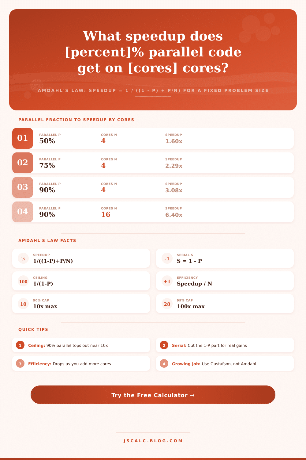
| 90% | 1.82x | 3.08x | 4.71x | 6.40x | 7.80x | 8.77x |
| 95% | 1.90x | 3.48x | 5.93x | 9.14x | 12.55x | 15.42x |
| 99% | 1.98x | 3.88x | 7.48x | 13.91x | 24.43x | 39.26x |
| 99.9% | 1.99x | 3.98x | 7.94x | 15.76x | 31.04x | 60.06x |
🎯Parallel Efficiency by Cores
| Parallel P | Eff at N=4 | Eff at N=16 | Eff at N=64 | Notes |
|---|---|---|---|---|
| 50% | 40.0% | 11.8% | 3.1% | Serial dominated |
| 75% | 57.1% | 21.1% | 5.97% | Wasted cores |
| 90% | 76.9% | 40.0% | 13.7% | Falls off fast |
| 95% | 86.9% | 57.1% | 24.1% | Better scaling |
| 99% | 96.9% | 86.9% | 61.3% | Near linear early |
| 100% | 100% | 100% | 100% | Ideal, unreal |
🚫Maximum Speedup Ceiling by Parallel Fraction
| Parallel P | Serial S = 1 - P | Ceiling 1/(1-P) | Even Infinite Cores |
|---|---|---|---|
| 50% | 0.50 | 2x | Capped at 2x |
| 75% | 0.25 | 4x | Capped at 4x |
| 90% | 0.10 | 10x | Capped at 10x |
| 95% | 0.05 | 20x | Capped at 20x |
| 99% | 0.01 | 100x | Capped at 100x |
| 99.9% | 0.001 | 1000x | Capped at 1000x |
⚖Amdahl vs Gustafson at a Glance
| Aspect | Amdahl's Law | Gustafson's Law |
|---|---|---|
| Problem size | Fixed workload | Grows with N |
| Question asked | Same job, more cores | Bigger job, same time |
| Speedup formula | 1/((1-P)+P/N) | N - S(N-1) |
| Scaling behavior | Diminishing returns | Near-linear |
| Upper limit | Hard cap 1/(1-P) | No fixed ceiling |
| Best used when | Latency of one task | Throughput, big data |
⚙Formula Breakdown
💡Parallel Scaling Tips
The Amdahl calculator will help you understand the impact of adding more cores. It relies on an equation from 1967 which illustrate the limits of hardware power. Enter your information into the calculator and it’ll run through the equation for you.
What remains are things that raw speed cannot solve. Strong scaling, or Amdahl’s Law, mean you get more processors without changing problem size. To illustrate this with an example, take a task that is ninety-five percent parallel and only five percent serial (meaning it must be done in order). If you increase your number of cores from one to eight, the parallel portion will become smaller; it’ll only do one-eighth of what it did before. But the serial part doesn’t decrease at all. The result is a speedup of around five point nine times. That’s not quite as good than you’d expect by just looking at number of cores! And that’s how much parallel computing comes up short of ideal.
How the Amdahl Calculator Works
So what is the result? The biggest effect of this law are the ceiling on how much speedup is possible. If the serial fraction is 50%, then the speedup converges to one over the serial fraction as the number of cores increases without limit. It all depends on the serial piece: if your workload is 90% parallel, it will never be faster than ten times no matter how many core you throw at it. If it’s 99% parallel, it’ll top out at one hundred times. This means there are diminishing returns in chasing higher numbers of cores. Eventually, you’ve squeezed out almost all parallelism and the remaining serial bottleneck limits everything, regardless of how many cores you use.
Use the calculator to work out this ceiling for yourself; then you know the limits before wasting money. After entering your inputs, four result cards summarise the outcome. The first (speedup) tells you how much faster the job will run with your selected core count. Dividing this by number of cores yields the second card (parallel efficiency), which describes how efficiently each processor is being used. In our case, an efficiency value of seventy-four percent indicates that average core is spending a quarter of its time idling while it waits for the serial bottleneck. Finally, the last card performs the opposite calculation: find me the least number of cores required to achieve my desired speedup, or inform me if the target lies beyond the impossible ceiling.
Real systems will have some coordination cost and thus can’t split off the parallel part of the work perfectly. There’s also inter-core communication, thread synchronization, and cache contention… And the more cores you have, the higher that overhead get. The tool has an optional overhead input that reduces the effective parallel fraction at each scale-up level. This pulls the predicted speedup back from under the textbook curve and reminds you that, in practice, measured scaling always lag behind theory. Seeing efficiency drop below half is a practical indicator to cease further scaling out and begin to optimize the serial code.
For example, imagine we have a video encode which is 95% parallel and takes 120 seconds to run on a single core. The tool would report that it ran in ~20 seconds (six times speedup) using eight cores. It would also show a maximum speedup of twenty regardless of scaling due to the five percent serial fraction. You ask it to target twenty-five times. It says, “sorry, your task has a five percent serial fraction, so there’s a lower bound to the speedup you can achieve.”
This provides a concrete answer to a vague hope. It turns this into a question you can make engineering decisions around. The underlying assumption of Amdahl’s Law (fixed problem size) is true for something like running one query or rendering one frame, where latency is what matters to you. But that paints a pessmistic view of another goal entirely. How about keeping the runtime fixed and allowing the problem to scale up with the machine? That’s the question Gustafson’s Law addresses. It says you’ll be able to get roughly linear scaling as long as bigger machines attack proportionally bigger problems.
The practical rule is simple: Use Amdahl when you have a fixed job and you need it done sooner; use Gustafson when you can expand the job and you need more throughput at the same time. Mistaking one for the other will lead to either disappointment or overspending. And so this calculator stays within the fixed-size model and alerts when the growing-workload case would apply instead.
This enables software engineers to determine if purchasing an additional machine is better than refactoring a serial hotspot. It helps data scientists predict how many cores a training run will require before it becomes inefficient. It also helps systems architects size their cluster relative to the limits imposed by their workloads.
At a glance, you have speedup and efficiency for common parallel fractions. Reference tables allows you to look up results for your particular situation. Presets let you load realistic scenarios from Monte Carlo simulations to database queries. Within seconds, you recieve defensible estimates of what will scale with parallelism, turning abstract theory into a hardware strategy you can use.