Disk IOPS Calculator
Estimate the random I/O an array can deliver. Enter drive type, drive count, RAID level and your read versus write mix, and the tool returns raw single-drive IOPS, total front-end IOPS the array serves, back-end functional IOPS after the RAID write penalty, and peak throughput in MB per second.
💾Real Array Presets
🔧Array Inputs
Sets a typical per-drive IOPS and latency you can override.
Count all data and mirror or parity members in the set.
Write penalty is the back-end ops per host write.
Fraction of I/O that is reads; write share fills the rest.
Random writes trigger the RAID penalty; reads do not.
Seek plus rotational; single-drive IOPS = 1000 / latency.
Enter a measured value (mainly for SSD/NVMe); 0 uses latency.
I/O size; throughput MB/s = IOPS x KB / 1024.
🔢Formula Snapshot
📊Drive Type Comparison Grid
| Drive Type | Single-Drive IOPS | Avg Latency | Interface | Typical Use |
|---|---|---|---|---|
| 7.2K SATA HDD | 75 to 100 | 11 to 13 ms | SATA | Bulk, archive, backup |
| 7.2K NL-SAS HDD | 80 to 110 | 10 to 12 ms | SAS | Capacity tiers |
| 10K SAS HDD | 125 to 150 | 6 to 8 ms | SAS | General virtualization |
| 15K SAS HDD | 175 to 210 | 4 to 6 ms | SAS | Transactional HDD tier |
| SATA SSD | 20K to 90K | 0.1 to 0.3 ms | SATA | Warm data, mixed use |
| SAS SSD | 50K to 200K | 0.08 to 0.2 ms | SAS | Enterprise flash |
| NVMe SSD | 100K to 1M | 0.02 to 0.1 ms | PCIe/NVMe | Databases, low latency |
🔑RAID Write Penalty Table
| RAID Level | Write Penalty | Fault Tolerance | Usable of N | Best For |
|---|---|---|---|---|
| RAID 0 | 1 | None | N | Scratch, cache |
| RAID 1 | 2 | 1 drive | N / 2 | Boot, small pairs |
| RAID 5 | 4 | 1 drive | N - 1 | Read-heavy files |
| RAID 6 | 6 | 2 drives | N - 2 | Large archive sets |
| RAID 10 | 2 | 1 per mirror | N / 2 | Write-heavy DB |
📋Latency to Single-Drive IOPS
| Access Latency | Drive IOPS | Matches | Notes |
|---|---|---|---|
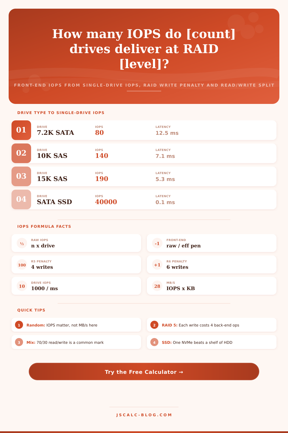
| 12.5 ms | 80 | 7.2K SATA | High seek + rotation |
| 7.1 ms | 141 | 10K SAS | Faster spindle |
| 5.3 ms | 189 | 15K SAS | Top HDD tier |
| 2.0 ms | 500 | Slow flash | Rarely spinning |
| 0.1 ms | 10000 | SATA SSD | Latency-dominated model breaks |
| 0.05 ms | 20000 | NVMe floor | Use measured IOPS instead |
⚙Formula Breakdown
💡Sizing Tips That Change the Math
If you aren’t working with storage every day, it’s confusing. Does your storage perform well? Well, how do you know?
You’ve got IOPS (how many individual operations finish per second) and you’ve got throughput (how much data does it move)? IOPS really matter for anything doing virtual machines and databases. Five hundred random reads per second won’t get you anywhere, even though your system might back up terabytes an hour in a row. Random versus sequential access matters because spinning disks and flash drives performs very differently when jumping between data on a platter or a controller matrix.
How to Measure Storage Speed
Those caps begin with latency: the time spent finding data determines how many operations can finish in one second. To figure out what’s possible from a single drive, divide 1,000 by the millisecond value of its average access time. That will give you a ballpark maximum number of I/Os per second.
For most drives, you’ll land somewhere between twelve and thirteen for a seven-thousand-two-hundred rpm sata drive. Faster fifteen-thousand RPM SAS drives will shave a few milliseconds off, bringing them down to five milliseconds or less, and top two hundred ops/sec. Latency is a whole different story when it comes to flash storage, there are no spinning heads here, and we’re dealing with a mechanical model where the measured IOPs numbers counts a lot more than theoretical latencies.
You can scale out with RAID 1. Now that you’ve seen what a single drive will do, scaling up appears straightforward, except when redundancy comes into play. Multiple drives offers multiplicative capacity by having their data stripped across them. That’s raw aggregate capacity. However, the RAID level imposes a tax on writes because it must maintain consistency between mirrors or parity.
It does this by writing the same information to multiple places, which is called the write penalty. You pay very little extra for reads. Writes forces the array to update multiple copies, which adds overhead. For example, a simple mirror doubles its write count per host request. Parity-based schemes like RAID five commonly use four back-end ops per front-end write. This process reads the old info and parity, then writes the new info and new parity. Even worse: RAID six is six ops. The penalty explains why capacity-oriented arrays is slow for write-heavy apps.
This blended math is calculated by the RAID multiplier applied against your read-to-write ratio. In our example of seventy percent reads and thirty percent writes, the effective cost per operation reduce greatly versus a pure write situation. The total raw IOPS of the array are divided by this weighted cost and shown as your actual front-end IOPS available to your servers. These then translate into megabytes per second using your chosen block size, connecting transaction speeds to bandwidth expectations.
Block size is an often-overlooked variable among most engineers who assume bigger blocks = better. This assumption does not hold for random I/O. There’s more to getting real world size right than simply nailing the number. Small bursts of writes gets absorbed by controller caches, hiding the mechanics of what lies below. Benchmark reports seldom show the invisible background load from deduplication and/or scrubbing tasks. To keep latency low under peak load it’s better to play it safe and stay at or below 70% use of whatever ceiling you calculate.
Don’t let disk space efficiency decide your RAID level. Use an access pattern to decide instead. For a transactional database, you’ll pay the price for parity RAID regardless of how many drives you stack. That’s how we go from guessing at storage to engineering: understanding those trade-offs. Rather than purchasing drive capacity, you purchase performance characteristics.
If it’s time to spin up a bunch of new virtual desktops, or if you’re archiving some cold data, you’ll know the difference between usable front-end IOPS and raw back-end operations, and avoid bottlenecks while saving money in the process. You don’t just want to fit your data; you also want to get it moving as soon as the user wants it. That’s when the rubber meets the road: balancing that equation of speed vs. Redundancy vs. Capacity.