CPU Instructions Per Second Calculator
Estimate raw CPU throughput as instructions per second from clock frequency, core count, and instructions per cycle. The tool multiplies frequency in Hz by IPC, cores, and an SMT efficiency factor to report theoretical peak IPS, then scales it by a workload factor for a more realistic effective figure, all shown as MIPS and GIPS with a per-core breakdown.
🧮Real CPU Throughput Presets
🖥CPU Specification Inputs
Peak uses IPC directly; CPI mode uses a cycles-per-instruction value instead.
Core clock in gigahertz. 1 GHz equals one billion cycles per second.
Physical cores available to run instructions in parallel.
Average instructions retired each clock cycle by one core.
Used in CPI mode. IPC equals 1 divided by this value.
1.0 means no SMT gain; 1.25 adds a typical 25 percent hyperthread boost.
Fraction of peak reached by real code. 0.5 means half of ideal throughput.
Sets the unit shown on the headline throughput card.
🔢Formula Snapshot
📋Clock and IPC to Peak Throughput
| Frequency | IPC | Single-Core IPS | Single-Core GIPS |
|---|---|---|---|
| 1 GHz | 1 | 1,000,000,000 | 1 GIPS |
| 2 GHz | 2 | 4,000,000,000 | 4 GIPS |
| 3 GHz | 3 | 9,000,000,000 | 9 GIPS |
| 3.5 GHz | 4 | 14,000,000,000 | 14 GIPS |
| 4 GHz | 4 | 16,000,000,000 | 16 GIPS |
| 4.5 GHz | 4 | 18,000,000,000 | 18 GIPS |
| 5 GHz | 5 | 25,000,000,000 | 25 GIPS |
| 2.5 GHz | 6 | 15,000,000,000 | 15 GIPS |
🔄IPC and CPI Relationship
| IPC | CPI = 1 / IPC | Meaning | Typical Case |
|---|---|---|---|
| 0.5 | 2.0 | Two cycles per instruction | Old or stalled core |
| 1.0 | 1.0 | One instruction each cycle | Simple scalar pipeline |
| 2.0 | 0.5 | Two instructions per cycle | Basic superscalar |
| 3.0 | 0.333 | Three per cycle | Wide mobile core |
| 4.0 | 0.25 | Four per cycle | Modern desktop core |
| 5.0 | 0.20 | Five per cycle | Leading wide core |
| 6.0 | 0.167 | Six per cycle | Very wide design peak |
🖥CPU Throughput Comparison Grid
| CPU Class | Clock GHz | Cores | IPC | Total GIPS | Per-Core GIPS |
|---|---|---|---|---|---|
| Embedded MCU | 1.0 | 1 | 1 | 1 | 1 |
| Budget laptop | 2.6 | 4 | 3 | 31.2 | 7.8 |
| Mobile phone | 2.8 | 8 | 3 | 67.2 | 8.4 |
| Mainstream desktop | 4.5 | 8 | 4 | 144 | 18 |
| High-end desktop | 5.0 | 16 | 5 | 400 | 25 |
| Workstation | 3.8 | 32 | 4 | 486.4 | 15.2 |
| Data center server | 2.5 | 64 | 4 | 640 | 10 |
| Single-thread champ | 5.0 | 1 | 5 | 25 | 25 |
📏Unit and Frequency Conversions
| Unit | Equals | In IPS | Note |
|---|---|---|---|
| 1 MHz | 1e6 cycles/s | 1e6 x IPC | Megahertz clock |
| 1 GHz | 1e9 cycles/s | 1e9 x IPC | Gigahertz clock |
| 1 MIPS | 1e6 instr/s | 1,000,000 | Million per second |
| 1 GIPS | 1e9 instr/s | 1,000,000,000 | Billion per second |
| 1 GIPS | 1000 MIPS | 1,000,000,000 | Scale by 1000 |
| 1 TIPS | 1e12 instr/s | 1,000,000,000,000 | Trillion per second |
⚙Formula Breakdown
💡Throughput Reality Tips
A trio of well-known specs on a spec sheet, frequency, IPC, and cores, condensed down into one number representing how many instructions of work a chip can do in a second. That’s called Instructions Per Second. It is typically expressed as GIPS (billions) or MIPS (millions).
It’s not the entire story about performance, but it’s a great place to start when comparing chips. It shows you roughly what a given clock speed gets you once you account for the width and degree of parallelism of that core. It also gives you something to use when sizing your workload.
What is Instructions Per Second?
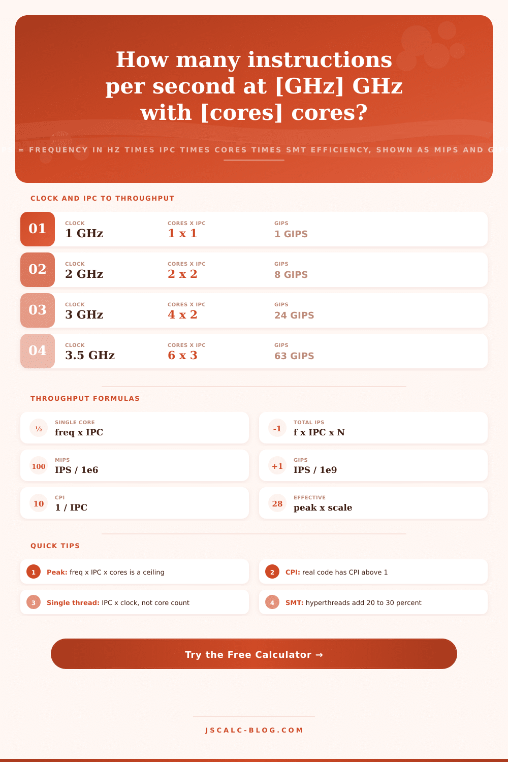
The number of machine instructions a processor executes in one second are called instructions per second, or IPS. A clocked core executing at frequency f perform f cycles per second. If it completes IPC instructions during each cycle, its throughput is simply f times IPC. Give it an IPC of 4 and a frequency of 4.5 GHz (which is 4.5 billion cycles per second), and we get a throughput of 18 billion instructions per second, which we write as 18 GIPS.
This is a throughput number. Throughput is how many instructions go through per unit time, not how quickly any individual instruction gets done. Note that today’s chips are not single-core. A core is a single unit that can execute instructions. Multiple cores runs in parallel; to calculate total throughput for a chip with N cores, just multiply a single-core throughput value by N. Thus if we have a 18 GIPS core running eight times on a single die, the theoretical peak throughput would of been 144 GIPS.
This calculation gets more complicated when considering simultaneous multithreading. If two threads share a single core, then it will stay busy during stalls where it might otherwise be idle, so there’s some additional utilization we model via an SMT efficiency factor greater than 1.0. The calculator shows that factor and lets you switch back-and-forth between a straight physical-core count and a version that factors in hyperthreading.
CPI counts the number of cycles required, on average, to complete one instruction. IPC does the opposite: it counts the number of instructions completed each cycle. Since they’re reciprocal, CPI = 1/IPC. So if your IPC is 1 then your CPI is 1.0. If your IPC is 4, your CPI is 0.25. People who work with profilers and architecture classes often tend to think in terms of cycles per instruction, so we’ve provided a CPI override mode where the per-core throughput is simply frequency/CPI. This allows you to enter in the CPI value directly from a perfcounter reading.
The conversation revolves around two scaled units. MIPS is a historic yardstick for today’s microcontrollers and older desktop chips that divides IPS by a million. GIPS is for moddern multi-core parts and divides IPS by a billion. Both convert IPS into smaller, more readable numbers. For our example above of 144 billion IPS, that’s 144,000 MIPS or more neatly stated as 144 GIPS. The tool shows both with the raw number for good measure… An embedded 1 GHz core will read out in MIPS; a 64-core server in GIPS (or even trillions of instructions per second).
All numbers above are peak… I.e., theoretical. They assume that all cores runs at their max instruction count every cycle, without interruption. That’s not real code. Memory bandwidth limits how quickly data can be fetched. Branch mispredictions flush out partially completed work. Cache misses stall the pipeline for dozens or even hundreds of cycles. In practice, actual CPI measured will float way higher than its ideal value; real-world throughput falls somewhere between 30 to 60 percent of peak, depending on what your mixed workload is. This translates directly to the scaling input. Set it to 0.5, and what was a 144 GIPS peak becomes just 72 GIPS, which is a much more realistic estimate for planning purposes. Think of peak as the ceiling and the scaled value as where you actualy get to live.
To summarize, the calculator provides four cards for each run. The GIPS and MIPS cards restate the overall throughput from the total throughput card in two standard scaled units (which will be adjusted for workload scaling, SMT, and cores). The third, the per-core IPS card, isolates what a single core would contribute (the metric governing single-threaded responsiveness). The total throughput card shows the whole-chip figure in your chosen unit, already adjusted by cores, SMT, and workload scaling. Below all of these is a breakdown panel showing the steps in between, such as frequency in hertz, effective throughputs, and peak throughputs. This tool also works as a check against your own math.
People tend to get fixated on the all-core total, but it doesn’t tell you anything about the feel of the system when running programs. For most of our everyday software, the program will run lightly threaded, riding on just one core. In that case, the per-core metric of frequency x IPC apply. If I have an IPC 5 core running at 5 GHz, that’s 25 GIPS single-threaded. This will beat the pants off a larger chip with less frequency (e.g., 2.5 GHz) and lower IPC (e.g., IPC 4), even though the latter stacks sixty-four cores into a massive overall number. Compare processor cards by weighing their total performance for parallel or batch work (such as simulation, compilation, rendering), and their per-core performance for interactive work.
These range from a 66 MHz retro chip at IPC 0.5 to a 3.0 GHz quad-core at IPC 2, a 4.5 GHz eight-core at IPC 4, a modern sixteen-core at IPC 5, and even a sixty-four-core server. Each loads the form and calculates instantly. This shows you how throughput scales with parallelism and width. Pick the closest preset to your chip, then tweak frequency, cores, IPC, SMT factor, and workload scaling to fit your exact case.
With the live breakdown plus the comparison grid and the IPC-to-CPI table, it provides a quick yet reliable estimate of CPU throughput in seconds. It clarifies the math so you no longer has to guess what those clock speeds actualy translate into for your workflow.