Bandwidth From Data Rate Calculator
Solve the required channel bandwidth in hertz from a target data rate using the Nyquist noiseless limit C = 2 B log2(M), the Shannon capacity C = B log2(1 + SNR), or a fixed spectral efficiency in bits per second per hertz, and see the matching symbol rate and achieved efficiency.
📡Choose a Method
🎯Real Link Presets
📝Channel Inputs
Selects which formula solves for bandwidth B.
Net bit rate the channel must carry.
Decimal units: 1 kbps = 1000 bps.
Signal levels per symbol; bits/symbol = log2(M).
Used for the Shannon capacity method.
Bits carried per second per hertz of bandwidth.
Extra bandwidth for FEC, guard band, and headers.
Display unit for the bandwidth card.
🔢Formula Snapshot
📋Modulation and Bits per Symbol
| Scheme | Order M | Bits per Symbol | Nyquist B for 100 Mbps |
|---|---|---|---|
| BPSK | 2 | 1 | 50.0 MHz |
| QPSK | 4 | 2 | 25.0 MHz |
| 8PSK | 8 | 3 | 16.7 MHz |
| 16QAM | 16 | 4 | 12.5 MHz |
| 32QAM | 32 | 5 | 10.0 MHz |
| 64QAM | 64 | 6 | 8.33 MHz |
| 256QAM | 256 | 8 | 6.25 MHz |
| 1024QAM | 1024 | 10 | 5.00 MHz |
📊SNR to Shannon Efficiency
| SNR (dB) | SNR (linear) | log2(1 + SNR) bps/Hz | B for 50 Mbps |
|---|---|---|---|
| 0 dB | 1.00 | 1.00 | 50.0 MHz |
| 3 dB | 2.00 | 1.58 | 31.6 MHz |
| 6 dB | 3.98 | 2.32 | 21.5 MHz |
| 10 dB | 10.0 | 3.46 | 14.4 MHz |
| 15 dB | 31.6 | 5.03 | 9.94 MHz |
| 20 dB | 100 | 6.66 | 7.51 MHz |
| 25 dB | 316 | 8.30 | 6.02 MHz |
| 30 dB | 1000 | 9.97 | 5.02 MHz |
| 35 dB | 3162 | 11.6 | 4.30 MHz |
📶Common Links: Rate and Bandwidth
| Link | Channel Bandwidth | Typical Data Rate | Modulation | Efficiency |
|---|---|---|---|---|
| Wi-Fi 802.11a/g | 20 MHz | 54 Mbps | 64QAM 3/4 | ~2.7 bps/Hz |
| LTE (single stream) | 20 MHz | 75 Mbps | 64QAM | ~3.8 bps/Hz |
| LTE-A 256QAM | 20 MHz | 100 Mbps | 256QAM | ~5.0 bps/Hz |
| DOCSIS 3.1 OFDM | 192 MHz | ~1.9 Gbps | 1024QAM | ~10 bps/Hz |
| 5G NR sub-6 | 100 MHz | ~600 Mbps | 256QAM | ~6.0 bps/Hz |
| Voiceband V.34 | 3.1 kHz | 33.6 kbps | QAM/TCM | ~10 bps/Hz |
| LoRa SF12 | 125 kHz | ~0.29 kbps | CSS spread | <0.01 bps/Hz |
🗃Modulation Comparison Grid
| Scheme | Order M | Bits/Symbol | Min SNR (dB) | Spectral Eff | Typical Use |
|---|---|---|---|---|---|
| BPSK | 2 | 1 | ~4 dB | 1 bps/Hz | Deep-space, control |
| QPSK | 4 | 2 | ~7 dB | 2 bps/Hz | Satellite, LTE edge |
| 8PSK | 8 | 3 | ~13 dB | 3 bps/Hz | DVB-S2, EDGE |
| 16QAM | 16 | 4 | ~16 dB | 4 bps/Hz | Wi-Fi, LTE mid |
| 32QAM | 32 | 5 | ~19 dB | 5 bps/Hz | Microwave backhaul |
| 64QAM | 64 | 6 | ~22 dB | 6 bps/Hz | Wi-Fi, cable, LTE |
| 256QAM | 256 | 8 | ~28 dB | 8 bps/Hz | LTE-A, 5G, DOCSIS |
| 1024QAM | 1024 | 10 | ~34 dB | 10 bps/Hz | Wi-Fi 6, DOCSIS 3.1 |
| 4096QAM | 4096 | 12 | ~40 dB | 12 bps/Hz | Wi-Fi 7 short range |
⚙Formula Breakdown
💡Bandwidth Planning Tips
Estimating a wireless link is kind of like stuffing a suitcase for a vacation that hasn’t happened yet. You know how many bits per second you need, but unless you has chosen a specific way to encode the signal, you don’t immediately know the bandwidth it will use in hertz. Enter our frequency calculation tool above.
Feed in your desired speed and modulation scheme, and the calculator does the rest. It spares you from trying to guess, convert, and multiply various coefficients. The answer reflects the minimum frequency slice required to keep data flowing without error.
How to Calculate Wireless Bandwidth
Yes, it’s little, but every bit counts when it comes to spectrum because it is a limited physical resource and a costly commodety. That’s where things get confusing, because many folks use bits-per-second (megabit) and hertz (megahertz) interchangeably. They’re not interchangeable. One 20 MHz-wide Wi-Fi channel may support dozens or even hundreds of megabits based off how densely it is packing that data.
Information theory is the link between the two… Specifically the theories developed by Claude Shannon and Harry Nyquist. Basically, their equations defines the theoretical upper limit of what is physically possible in a particular scenario. When applied, it use three timeless relationships. It then solves for bandwidth. This lets you clearly understand how much of the spectrum any modulation choice uses.
As Nyquist demonstrated, in an ideal noise free universe, your maximum symbol rate is twice the bandwidth. If signal has sufficient numbers of distinct levels (called M), then each symbol carries some number of bits. The capacity formula says C equals two B log base two of M. To solve for bandwidth, we rearrange to get B equals C divided by two log base two of M. You desire one hundred megabits per second with sixty four QAM. Log base two of sixty-four is six. So the needed bandwidth is one hundred million divided by twelve. It is about eight point three-three megahertz. This is the ideal minimum, assuming zero interference.
The Nyquist limit is optimistic at best. Noise are present in all real channels. And Shannon filled in the gap with what he called his capacity theorem. C equals B log base two of one plus SNR. That’s an absolute upper bound on performance that cannot be exceeded, no matter how clever engineer may be. Plug in your target speed, and you get B equals C divided by log base two of one plus SNR. Now, note that signal-to-noise ratio is typically expressed in dB, so the calculator converts that to a linear power ratio. Twenty five dB represents a linear ratio of approximately 316. This gives a theoretical efficiency of about eight point three bits per second per hertz.
So what about when you don’t care about spectral efficiency? You already know that a given tech can deliver some number of bits per hertz per stream. For example, LTE with sixty-four QAM comes in around three point eight bits per second per hertz per stream. DOCSIS thirty-one with one thousand twenty-eight QAM is closer to ten bits per second per hertz. Then it’s simple arithmetic. B equals data rate divided by eta. That’s how the spectral efficiency method works.
If I want six hundred megabits and I am getting six bits per second per hertz, then a one-hundred-megahertz channel immediately falls out. This is the fastest route to sanity-checking your spectrum allocation without going deep into modulations.
The other thing reported in all these results is baud, or symbol rate. That’s important because eventually bandwidth goes back to how quickly symbols appears on the channel. Baud = bitrate / log base two of M. If you have sixty-four QAM at a hundred megabits per second, then each symbol represent six bits. Six bits times 16 million symbols per second is roughly sixteen point six-seven megabaud. Why keep track of bits per second separately from baud? Because it avoids a common error when doing link budgets. Bits per second equal baud if and only if M=2, which means binary signaling. With any higher order scheme, the bit rate is more than the baud rate by the number of bits per symbol.
Those figures are the theoretical minimums: Nyquist and Shannon. They require perfect conditions (no framing, ideal pulse shaping). Real-world systems include protocol headers, pilot tones, guard intervals, and forward error correction. These all eat up spectrum. To account for this in real life, you can specify an overhead percentage on the calculator, which will increase the ideal bandwidth by fifteen to twenty percent. That’s reflective of reality. With a twenty-megahertz Wi-Fi channel, only roughly sixteen point six megahertz of that are dedicated to usable data subcarriers. The rest is used by pilots and guard bands. Add in overhead and you transform an academic number into something you could of use when planning.
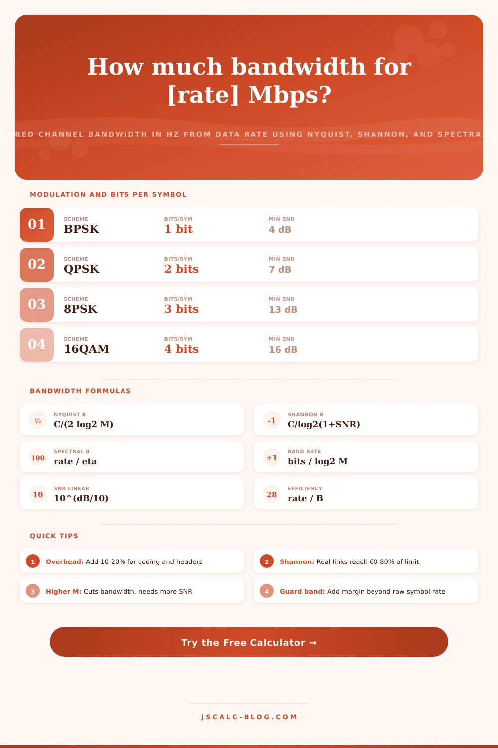
To make the numbers concrete, there are some tables under the calculator. One is the modulation table, which shows how many bits are in each symbol. What’s the Nyquist bandwidth required to deliver a hundred megs/sec at that rate? You can see how 1,024 QAM reduces the demand by a factor of ten compared too BPSK.
Another table is the SNR table: converting SNR in dB to a linear ratio and to Shannon efficiency. That way, you can easily compare bandwidth savings from a clean signal. A third is a common links table comparing various common schemes (LoRa, voiceband modems, DOCSIS, LTE, Wi-Fi). The comparison grid pairs each modulation order with its minimum SNR, spectral efficiency, and typical deployment so you can match a scheme to your link margin.
So you should of be able to match a scheme to your link margin. Is there a frequency channel to choose between? Do you need a data rate to size a satellite downlink or plan a microwave backhaul hop? Are you prepping for a communications exam or just wondering how much spectrum a gigabit connection require?
Enter some initial value like Wi-Fi sixty-four QAM or LTE two hundred fifty-six QAM. Select one of three methods, Nyquist, Shannon, and spectral efficiency, to compare results. Observe each step in the breakdown panel. What emerges is a clear and reliable bandwidth calculation, honoring both the theoretical limits of information theory and the real-world overhead of an operational radio. You’ll have order restored to your packing problem.