Bandwidth Delay Product Calculator
Compute the bandwidth delay product with BDP = bandwidth times round-trip time, then size the TCP window and receive buffer needed to keep a long fat pipe full. See BDP in kilobytes and megabytes, the minimum window, packets in flight for your MSS, and the link utilization a configured window would achieve.
📡Real Network Path Presets
📝Link and TCP Inputs
Usable throughput of the bottleneck link.
Bits are counted as 1000-based (1 Mbps = 1,000,000 bit/s).
Ping time there and back along the full path.
TCP payload per packet, typically 1460 on Ethernet.
Current send or receive window. Used for utilization.
Bytes are 1024-based (1 KB = 1024 bytes).
Controls rounding on every result card.
🔢Formula Snapshot
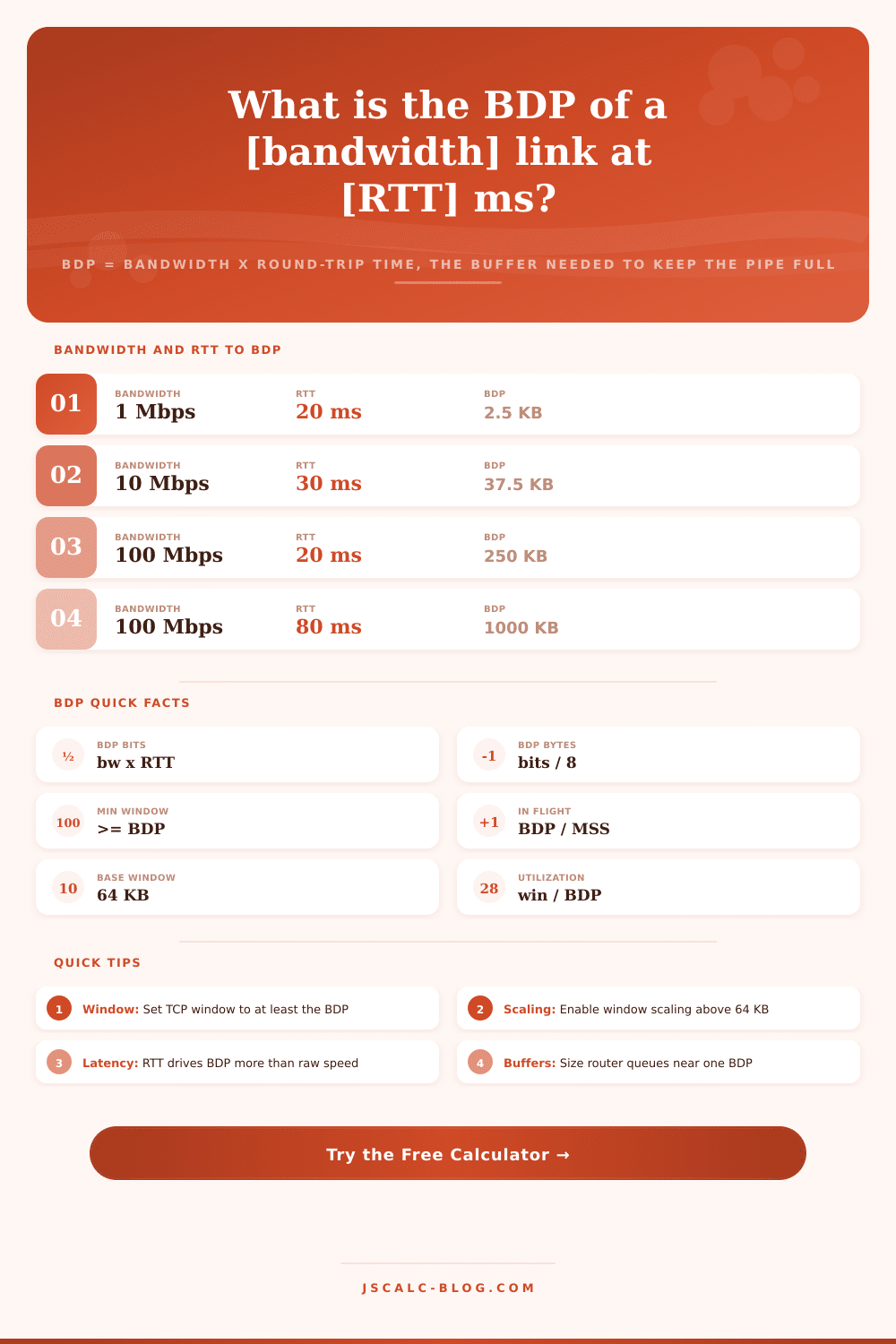
📈Bandwidth and RTT to BDP Examples
| Bandwidth | RTT | BDP (bytes) | Reads As |
|---|---|---|---|
| 1 Mbps | 20 ms | 2,500 B | 2.44 KB |
| 10 Mbps | 30 ms | 37,500 B | 36.6 KB |
| 100 Mbps | 20 ms | 250,000 B | 244 KB |
| 100 Mbps | 80 ms | 1,000,000 B | 977 KB |
| 1 Gbps | 20 ms | 2,500,000 B | 2.38 MB |
| 1 Gbps | 100 ms | 12,500,000 B | 11.9 MB |
| 50 Mbps | 600 ms | 3,750,000 B | 3.58 MB |
| 10 Gbps | 10 ms | 12,500,000 B | 11.9 MB |
🔧TCP Window Scale Factors
| Scale Factor | Multiplier 2^n | Max Window | Fits BDP Up To | Typical Use |
|---|---|---|---|---|
| 0 | 1x | 64 KB | 64 KB | LAN, low RTT |
| 1 | 2x | 128 KB | 128 KB | Fast metro WAN |
| 2 | 4x | 256 KB | 256 KB | Regional 100M |
| 3 | 8x | 512 KB | 512 KB | National WAN |
| 4 | 16x | 1 MB | 1 MB | Transatlantic |
| 6 | 64x | 4 MB | 4 MB | Long-haul 1G |
| 7 | 128x | 8 MB | 8 MB | GEO satellite |
| 9 | 512x | 32 MB | 32 MB | 1G intercontinental |
🌐Real Path Examples With BDP
| Path Type | Bandwidth | RTT | BDP | Window Needed |
|---|---|---|---|---|
| Gigabit LAN | 1 Gbps | 1 ms | 122 KB | 128 KB |
| Office WAN | 100 Mbps | 40 ms | 488 KB | 512 KB |
| Fiber to cloud | 1 Gbps | 25 ms | 2.98 MB | 4 MB |
| 4G LTE mobile | 50 Mbps | 60 ms | 366 KB | 512 KB |
| 5G broadband | 300 Mbps | 25 ms | 916 KB | 1 MB |
| GEO satellite | 50 Mbps | 600 ms | 3.58 MB | 4 MB |
| LEO Starlink | 150 Mbps | 45 ms | 824 KB | 1 MB |
| 10G data center | 10 Gbps | 0.5 ms | 610 KB | 1 MB |
🗃Link Comparison Grid
| Link | Bandwidth | RTT | BDP (KB) | BDP (MB) | Window Needed |
|---|---|---|---|---|---|
| Home ADSL | 16 Mbps | 30 ms | 58.6 KB | 0.06 MB | 64 KB |
| Gigabit LAN | 1 Gbps | 1 ms | 122 KB | 0.12 MB | 128 KB |
| 100M Metro | 100 Mbps | 10 ms | 122 KB | 0.12 MB | 128 KB |
| 100M National | 100 Mbps | 80 ms | 977 KB | 0.95 MB | 1 MB |
| 1G Transatlantic | 1 Gbps | 90 ms | 10,986 KB | 10.7 MB | 16 MB |
| 4G LTE | 50 Mbps | 60 ms | 366 KB | 0.36 MB | 512 KB |
| 5G mmWave | 1 Gbps | 15 ms | 1,831 KB | 1.79 MB | 2 MB |
| GEO Satellite | 50 Mbps | 600 ms | 3,662 KB | 3.58 MB | 4 MB |
| LEO Starlink | 150 Mbps | 45 ms | 824 KB | 0.80 MB | 1 MB |
| 10G DC Fabric | 10 Gbps | 0.5 ms | 610 KB | 0.60 MB | 1 MB |
⚙Formula Breakdown
💡BDP Tuning Tips
How fast can something move across a long-distance network? It’s a simple question with an answer provided by this page: the bandwidth delay product (BDP) calculator. To maintain a full-link transfer, you have to push as many bits down the wire in one shot as possible.
The number to calculate is called the bandwidth delay product. It’s the link bandwidth times the round-trip time. Get this calculation correct and your stream flows at full-line rates. Get it wrong and a gigabit link crawls, even though the connection’s rated for maximum throughput.
Understanding Bandwidth Delay Product
Imagine if you have a pipe used for transporting water. It will have some amount of water based off its diameter and length. Even if they is moving the same amount of water, a longer pipe has more water than a shorter one. Similarly, a network path are like this. Bandwidth is the diameter, round-trip time is the length, and BDP is how much total data the path can contain without acknowledging the first byte.
In other words, the BDP in bits equals (bandwidth in bits per second) * (RTT in seconds), then you divide by eight to get it in bytes. At any given moment, a 1 Gbps link with 20 milliseconds of round trip will have about 2.38 megabytes in flight.
The TCP window size represent how much data a sender is allowed to have sent out but not acknowledged. If the window is smaller than the BDP, the sender empties its allowance and stalls, idle, until the first acknowledgment completes its round trip. Since TCP is a reliable protocol, the sending host will only have a certain amount of unacknowledged data in flight. The window is the amount. When this is less than the BDP, then the sender exhausts their allowance and stops until an acknowledgement makes it back after one round trip. During each of these pauses, the link is sitting there half-full. You want to keep the pipe full.
This means the receive window, the send window, and the socket buffers behind them should be big enough to hold at least one BDP. The calculator above does the math for you and reports that number right back to you so you can size your buffers from something other than a wild guess.
Back in the day, when the TCP header was defined, it allocated a mere sixteen bits for its window field, limiting it to no more than 65,535 bytes, roughly 64 kilobytes. In today’s world, on a fast path, that limit’s too small. Our 2.38 megabyte example requires nearly forty times as large a base window. The solution? TCP’s window scaling option effectively multiplies the advertised window size by two raised to some agreed-upon scale factor. The tool calculates the necessary scale factor for your path by finding the minimum power of two that raises the base window above your BDP. (For a 2.5 megabyte BDP, the scale factor is six; that gives you a 4 megabyte usable window and comfy headroom.)
For each calculation, we get four cards: First, the BDP (in kilobytes or megabytes), followed by an exact count of bits and bytes below that. Second, we get the recommended minimum buffer and window, rounded up to the nearest power of two, and the scale factor used to get there. Third, packets in flight is BDP divided by max segment size, which tells you how many segments are on the wire at any given time. Fourth, link use, i.e., what percentage of the pipe is your configured window filling? If it’s low, you’re not starving the connection.
Take our example, a 90-millisecond round-trip for a transatlantic 1 Gbps circuit: 90 million bits = 10.7 megabytes. At a default window size of just 64 KB we’ll be using less than 0.6 percent of the bandwidth. In other words, it’s as if you’ve throttled that gigabit circuit down to a few megabits per second. For a transatlantic 1 Gbps circuit with a 90 millisecond round trip, increasing your window to 16 megabytes lets the transfer run at line rate. All of these figures, including the maximum throughput you’d achieve with a tiny window, are surfaced in the calculator; you quickly see the price paid for an insufficiently-sized buffer.
The key insight here is that bandwidth and RTT enter the product symmetrically: doubling either one doubles the BDP. That’s why satellite links are so demanding. Geostationary hops add about 600 milliseconds of round-trip delay. Even with a modest 50 Mbps satellite link, we have a 3.58 megabyte BDP; bigger than many gigabit terrestrial paths.
Why does moving a server closer to its users often make throughput better? Because it improves both sides of the equation. You see this laid out in the reference table on the page. It compares LAN, WAN, mobile and satellite paths so you can easily compare the effect side by side.
Host TCP tuning isn’t all there is to the BDP. Historically, one BDP was the rule of thumb for sizing queues in routers and switches. This allows them to buffer enough data for a full round trip during congestion and avoid dropping packets too early. If you undersize the router buffers things go wrong: lots of losses and throughput collapse. If you grossly oversize them, things goes wrong too. The queues fill up. Latency grows. Buffer bloat. Knowing the BDP for the paths a device serves provides a principled starting point for both host buffers and network equipment.
Pick a scenario that’s similar to yours: 4G mobile link? Gigabit LAN? Geostationary satellite hop. Tweak the bandwidth, RTT, and your configured window to reflect what’s actualy happening. Change the delay some more, and observe what happens to utilization and the recommended window. For troubleshooting a slow backup over a WAN, or even tuning a data transfer node, the tool will make what’s normally an abstract formula concrete, the width of the pipe isn’t all there is; it’s also about how much data it can hold while it waits for the echo to return.
You should of checked your settings earlier. Use different than you think for a largger window. Most people finds it difficultly.