Hamming Distance Calculator
Compare two equal-length words position by position to count the differences. Enter binary, hexadecimal, or plain text to get the Hamming distance, similarity percentage, matching positions, and the error-detecting and error-correcting power that distance gives a code under the rule d = 2t + 1.
📏Choose a Mode
🎯Real Word-Pair Presets
📝Word Inputs
Binary and hex compare bits; text compares characters.
Symbol mode counts differing characters, not bits.
The first of the two equal-length words to compare.
Must be the same length as String A after cleaning.
Smallest Hamming distance between any two valid codewords.
Total bits per codeword, for the rate note only.
Displays both words stacked with differing positions marked.
In text mode, treat A and a as different characters.
Aligned comparison (mismatches highlighted)
🔢Formula Snapshot
📐How Distance Is Counted
| Input Type | Compared By | Rule | Example Pair | Distance |
|---|---|---|---|---|
| Binary | Bit by bit | popcount(A XOR B) | 1011 vs 1001 | 1 |
| Hexadecimal | Nibble to bits | XOR then count 1s | 0xFF vs 0x0F | 4 |
| ASCII text | Char by char | count A[i] != B[i] | karolin/kathrin | 3 |
| Binary (inverse) | Bit by bit | every bit flips | 1010101/0101010 | 7 |
| Decimal digits | Digit by digit | count differing | 2173896/2233796 | 3 |
| Identical | Any basis | distance is zero | 10110 vs 10110 | 0 |
🛡Minimum Distance to Error Capability
| d(min) | Errors Detected (d-1) | Errors Corrected floor((d-1)/2) | Meaning |
|---|---|---|---|
| 1 | 0 | 0 | No protection |
| 2 | 1 | 0 | Detect single error |
| 3 | 2 | 1 | Single-error correcting |
| 4 | 3 | 1 | SECDED style |
| 5 | 4 | 2 | Double-error correcting |
| 6 | 5 | 2 | Correct 2, detect 5 |
| 7 | 6 | 3 | Triple-error correcting |
| 8 | 7 | 3 | Correct 3, detect 7 |
🗄Word-Pair Comparison Grid
| Word A | Word B | Length | Distance | Similarity | Correctable |
|---|---|---|---|---|---|
| 1011 | 1001 | 4 bits | 1 | 75% | 0 |
| karolin | kathrin | 7 chars | 3 | 57.1% | 1 |
| 2173896 | 2233796 | 7 digits | 3 | 57.1% | 1 |
| 0xFF | 0x0F | 8 bits | 4 | 50% | 1 |
| 10110 | 10110 | 5 bits | 0 | 100% | 0 |
| 1010101 | 0101010 | 7 bits | 7 | 0% | 3 |
| toned | roses | 5 chars | 3 | 40% | 1 |
| GATTACA | GACTATA | 7 bases | 3 | 57.1% | 1 |
| 00000000 | 11111111 | 8 bits | 8 | 0% | 3 |
| 1100110 | 1100000 | 7 bits | 2 | 71.4% | 0 |
🧩Known Codes and Their Minimum Distance
| Code | n, k | d(min) | Corrects | Common Use |
|---|---|---|---|---|
| Repetition (3,1) | 3, 1 | 3 | 1 error | Simple redundancy |
| Hamming (7,4) | 7, 4 | 3 | 1 error | RAM and links |
| Extended Hamming (8,4) | 8, 4 | 4 | 1 error, detect 2 | SECDED memory |
| Single parity (8,7) | 8, 7 | 2 | 0 (detect 1) | Serial links |
| Reed-Muller (16,5) | 16, 5 | 8 | 3 errors | Deep-space Mariner |
| Golay (23,12) | 23, 12 | 7 | 3 errors | Voyager spacecraft |
| ISBN-10 checksum | 10, 9 | 2 | 0 (detect 1) | Book numbers |
⚙Formula Breakdown
💡Practical Distance Tips
If we have two equal-length words, then the Hamming distance is a measure of their position differences. Sounds like a basic high-school math problem. But this is also at the center of nearly all of todays error-correcting codes in computing.
In 1950, fed up with computers halting at the slightest bit error, Richard Hamming proposed a new way to think: Why not make computers continue to run, fixing themselves along the way? The calculator can do the counting for us, but what does that count mean? How much redundancy should our data realy require to survive? It’s about knowing how much data should be added so there’s enough redundancy to fight off noise.
What Is Hamming Distance?
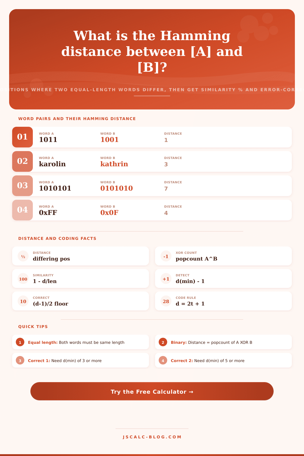
If you’re feeding it binary strings, then it counts the number of bits that don’t match up from one string to another. Mathematically speaking this is the same as performing a bitwise XOR between words and then counting the number of ones that result. That operation is called population count or popcount. If you want, compare the word 1011 with 1001. Their XOR would be 0010. There’s only a single one there so we say distance between these two words is one.
Now, when you have hexadecimal input, it expands them into four-bit nibbles and then compares them. In text mode it doesn’t work like that. Instead of comparing all the bits together, it just compares each character separately. Hence Karolin and Kathrin get a distance of three. They all match except for the fourth, fifth, and sixth letters. It makes sense because each character carries a lot more information than a single bit does. When you change a letter you normaly end up changing multiple underlying bits at once.
The problem is that there’s no way to tell from distance how far apart they actualy are: Three may seem like a lot if you’re measuring between two paragraphs, but not so much if you’re measuring in terms of two bytes. That’s where similarity comes into play. To calculate it, take the distance divided by the length and subtract one. Multiply that by one hundred. A distance of three out of five characters mean a forty percent similarity. A distance of one out of four bits result in a seventy-five percent match. What about the number of matching positions? Just do the length minus the distance.
The key point here is that all these calculations starts with a length test. Words of different lengths has no hamming distance. Try entering a six-symbol word and compare it to a seven-symbol word. The tool will flag this as a mismatch. It will nudge you towards edit distance, which is correct measure if you allow both insertions and deletions instead of substitutions.
This metric gets realy interesting because it comes from coding theory. Imagine a set of valid codewords sprinkled across the space of all possible patterns of bits. How far away are the nearest two valid codewords? This is called minimum Hamming distance of the code (denoted d(min)). If no two valid codewords are closer than d(min), then changing fewer than d(min) bits can never turn one valid codeword into another.
And there we have it. One simple geometric fact produces two classic results. The code will detect up to d(min)-1 errors. It will also corrects up to floor((d(min)-1)/2) errors. These is computed the instant you enter a minimum distance into the second mode of the calculator. You can then click into that Code Detect and Correct mode and play around with the design rule itself.
A code must have a minimum distance of at least 2t + 1 if it’s going to correct up to t independent errors per codeword. So for example, correcting just one bit error require a minimum distance of three. That is what happens with the famous Hamming seven-four code, which has a distance of three and corrects one error in each of the seven bits in a block. Two bit errors would require a distance of five. Three errors would require a distance of seven. This brings us to the famous Golay code used on the Voyager spacecraft to send their signals all those years.
Input a minimum distance and the cards will instantly show you how many errors that code will detect and correct. You can size your redundancy to account for actual level of noise you might reasonably expect.
Hamming distance crops up in more than just the pages of textbook coding theory. If you have two things to compare that are both the same length, then it’s all over the place. It pops up in bioinformatics, where we use it to compare DNA sequences of the same length. It shows up in computer memory. There, we use variants based off distance-four Hamming codes (SECDED) to detect and correct single-bit flips caused by cosmic rays. It shows up in machine learning, where it serves as a measure for comparing hashes and other binary feature vectors. And even spell checkers and fuzzy string matching rely on it when the set of candidate words is the same length.
The definition is simple, a really basic mathematical thing used in many different places. When you couple that with a convenient calculator that explains the coding-theory meaning of the number, you can go from a raw number back to an informed decision about your design. Not knowing how much you’re protected but wanting to know goes away. Knowing exactly what kinds of errors you’re protected against and designing for them take its place. It brings that 1950 frustration into the present with a clear mathematical solution to the problem. You should of used it sooner.